Premade Couplers via Inverse Design
Using an inverse design optimizer and SCEE, various power splitting
couplers at various splitting ratios have been designed and saved for
future use. These can be loaded using
SiPANN.scee_opt.premade_coupler module. We’ll go through how to load
them here.
import numpy as np
import matplotlib.pyplot as plt
from SiPANN import scee_opt, scee

def pltAttr(x, y, title=None, legend='upper right', save=None):
    if legend is not None:
        plt.legend(loc=legend)
    plt.xlabel(x)
    plt.ylabel(y)
    if title is not None:
        plt.title(title)
    if save is not None:
        plt.savefig(save)
Crossover
Premade couplers can be loaded via the
SiPANN.scee_opt.premade_coupler function. It takes in a desired
percentage output of the throughport. The only percentages available are
10, 20, 30, 40, 50, and 100 (crossover). It returns a instance of
SiPANN.scee.GapFuncSymmetric with all it’s usual functions and
abilities, along with the coupler length in nanometers.
If you desire other ratios, see the tutorial on
SiPANN.scee_opt.make_coupler, where the inverse design optimizer can
be used to make arbitrary splitting ratios.
crossover, length = scee_opt.premade_coupler(100)
crossover.gds(view=True,extra=0,units='microns')
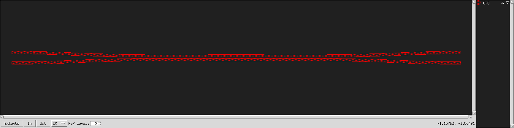
crossover
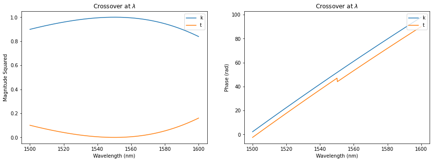
wavelength = np.linspace(1500, 1600, 500)
k = crossover.predict((1,4), wavelength)
t = crossover.predict((1,3), wavelength)

plt.figure(figsize=(15,5))
plt.subplot(121)
plt.plot(wavelength, np.abs(k)**2, label='k')
plt.plot(wavelength, np.abs(t)**2, label='t')
pltAttr('Wavelength (nm)', 'Magnitude Squared', 'Crossover at $\lambda \approx 1550nm$')
plt.subplot(122)
plt.plot(wavelength, np.unwrap(np.angle(k)), label='k')
plt.plot(wavelength, np.unwrap(np.angle(t)), label='t')
pltAttr('Wavelength (nm)', 'Phase (rad)', 'Crossover at $\lambda \approx 1550nm$')
30/70 Splitter
For further demonstration, we also load a 30/70 splitter.
splitter, length = scee_opt.premade_coupler(30)
splitter.gds(view=True,extra=0,units='microns')
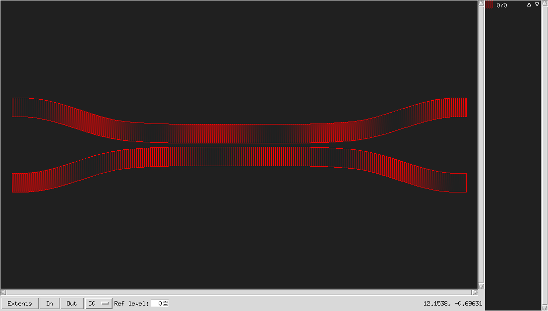
splitter
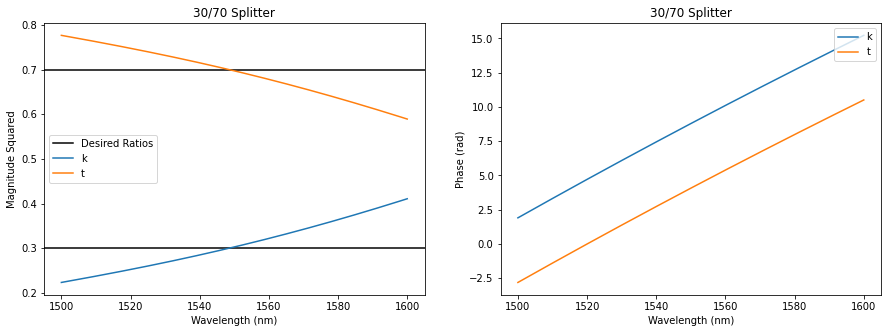
wavelength = np.linspace(1500, 1600, 500)
k = splitter.predict((1,4), wavelength)
t = splitter.predict((1,3), wavelength)

plt.figure(figsize=(15,5))
plt.subplot(121)
plt.axhline(.3, c='k', label="Desired Ratios")
plt.axhline(.7, c='k')
plt.plot(wavelength, np.abs(k)**2, label='k')
plt.plot(wavelength, np.abs(t)**2, label='t')
pltAttr('Wavelength (nm)', 'Magnitude Squared', '30/70 Splitter', legend='center left')
plt.subplot(122)
plt.plot(wavelength, np.unwrap(np.angle(k)), label='k')
plt.plot(wavelength, np.unwrap(np.angle(t)), label='t')
pltAttr('Wavelength (nm)', 'Phase (rad)', '30/70 Splitter')
If you’d like this tutorial as a jupyter notebook, it can be found on github, here