Inverse Design using SCEE
Do to how fast SCEE is, inverse design of power splitting directional
couplers can be achieved via an optimizer. This has been implemented and
can be used via the SiPANN.scee_opt module, speficially the
make_coupler function. It implements a global optimization, then a
local optimization to best find the ideal coupler.
This is done by defining the length of the coupler and various control points along the coupler as parameters that our optimizer can choose that result in a \(\kappa\) closest to \(\kappa_{goal}\). The coupler is then defined using the control points plugged into a Bezier Curve. Note that the Bezier curve defined by the control points is the gap between waveguides, not the geometry of the waveguides themselves. However, since each of these directional couplers is symmetric the inner boundary of the waveguides are just half of the gap.
Further, for our objective function, we compute \(\kappa\) for a sweep of wavelength points using SCEE, and then calculate the MSE by comparing it to \(\kappa_{goal}\). Various constraints are also put on the coupler, like ensuring the edges of the coupler are far enough apart and making sure there’s no bends that are too sharp. To learn more about the process, see [INSERT PAPER WHEN PUBLISHED].
import numpy as np
import matplotlib.pyplot as plt
from SiPANN import scee_opt, scee

def pltAttr(x, y, title=None, legend='upper right', save=None):
    if legend is not None:
        plt.legend(loc=legend)
    plt.xlabel(x)
    plt.ylabel(y)
    if title is not None:
        plt.title(title)
    if save is not None:
        plt.savefig(save)
Wavelength Sweep
Most of the defaults parameters for SiPANN.scee_opt.make_coupler
have been set because they work well, so if you don’t know what you’re
doing, it’s generally best to stick with them. Here we make a coupler
with 25% of the light coming out of the cross port. It will return an
instance of SiPANN.scee.GapFuncSymmetric, the control points chosen,
and the final length of the coupler.
The number of points passed into waveSweep is the one that affects
how long the optimizer takes the most. We pass in 2 points. This will
cause the optimizer to use the endpoints of our wavelength sweep when
evaluating the objective function. This is generally sufficient since
the response is usually either increasing or decreasing everywhere, so
trying to push the endpoints to our desired ratio is enough.
width = 500
thickness = 220
coupler, gap_pts, length = scee_opt.make_coupler(goalK=.25, verbose=1,
                                                 width=width, thickness=thickness,
                                                 waveSweep=np.array([1500,1600]), maxiter=15000)
LOCAL, MSE: 0.0267, Mean currK: 0.2864: 50%|█████ | 15001/30000 [42:58<38:09, 6.55it/s]
We can easily save it to an npz file for later use using
SiPANN.scee_opt.save_coupler
scee_opt.save_coupler(width, thickness, gap_pts, length, "split_25_75.npz")
And then reload it using the SiPANN.scee_opt.load_coupler. This will
return us an instance of SiPANN.scee.GapFuncSymmetric.
coupler, length = scee_opt.load_coupler("split_25_75.npz")
And we’ll check what it looks like and make sure it performs as we anticipated.
coupler.gds(view=True,extra=0,units='microns')
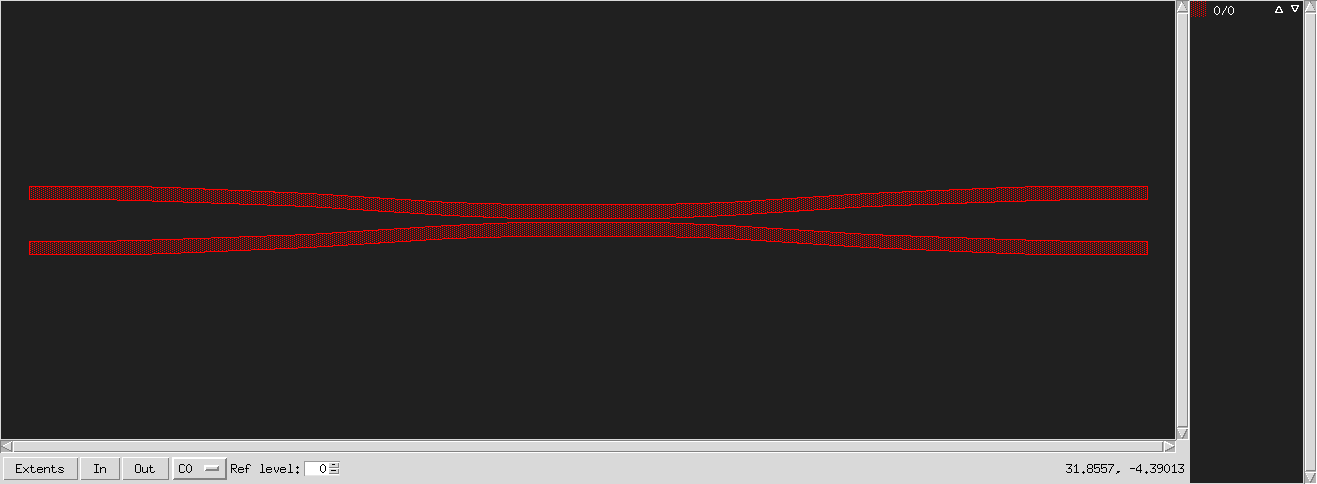
coupler
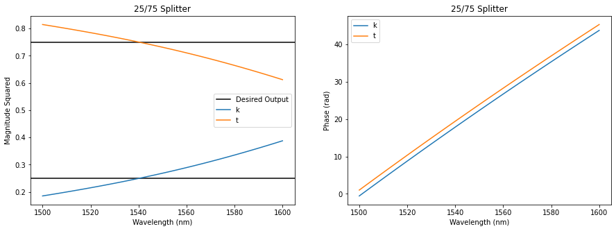
wavelength = np.linspace(1500, 1600, 100)
k = coupler.predict((1,4), wavelength)
t = coupler.predict((1,3), wavelength)

plt.figure(figsize=(15,5))
plt.subplot(121)
plt.axhline(.25, c='k', label="Desired Output")
plt.axhline(.75, c='k')
plt.plot(wavelength, np.abs(k)**2, label='k')
plt.plot(wavelength, np.abs(t)**2, label='t')
pltAttr('Wavelength (nm)', 'Magnitude Squared', '25/75 Splitter', legend='best')
plt.subplot(122)
plt.plot(wavelength, np.unwrap(np.angle(k)), label='k')
plt.plot(wavelength, np.unwrap(np.angle(t)), label='t')
pltAttr('Wavelength (nm)', 'Phase (rad)', '25/75 Splitter', legend='best')
For your convenience, this has been done for a variety of splitting
ratios already and they all can be loaded using
SiPANN.scee_opt.premade_coupler. To learn more about how to use that
see the tutorial on Premade Couplers via Inverse Design.
Single Wavelength
If we desire a specific wavelength to have a ratio, we can achieve this
by making waveSweep only have one element. This causes only a single
wavelength to be optimized (and a solution is generally found very
quickly). This enforces nothing on any other wavelengths, so it’s
possible that it will be significantly different than the desired ratio
even at close wavelengths.
For an example, we show this for \(\lambda=1530nm\) and a ratio of 45%.
width = 500
thickness = 220
coupler, gap_pts, length = scee_opt.make_coupler(goalK=.45, verbose=1,
                                                 width=width, thickness=thickness, maxiter=30000,
                                                 waveSweep=np.array([1530]))
scee_opt.save_coupler(width, thickness, gap_pts, length, "split_45_55_1530.npz")
LOCAL, MSE: 0.1523, Mean currK: 0.1832: 18%|█▊ | 10975/60000 [18:09<1:31:59, 8.88it/s]
coupler, length = scee_opt.load_coupler("split_45_55_1530.npz")
coupler.gds(view=True,extra=0,units='microns')
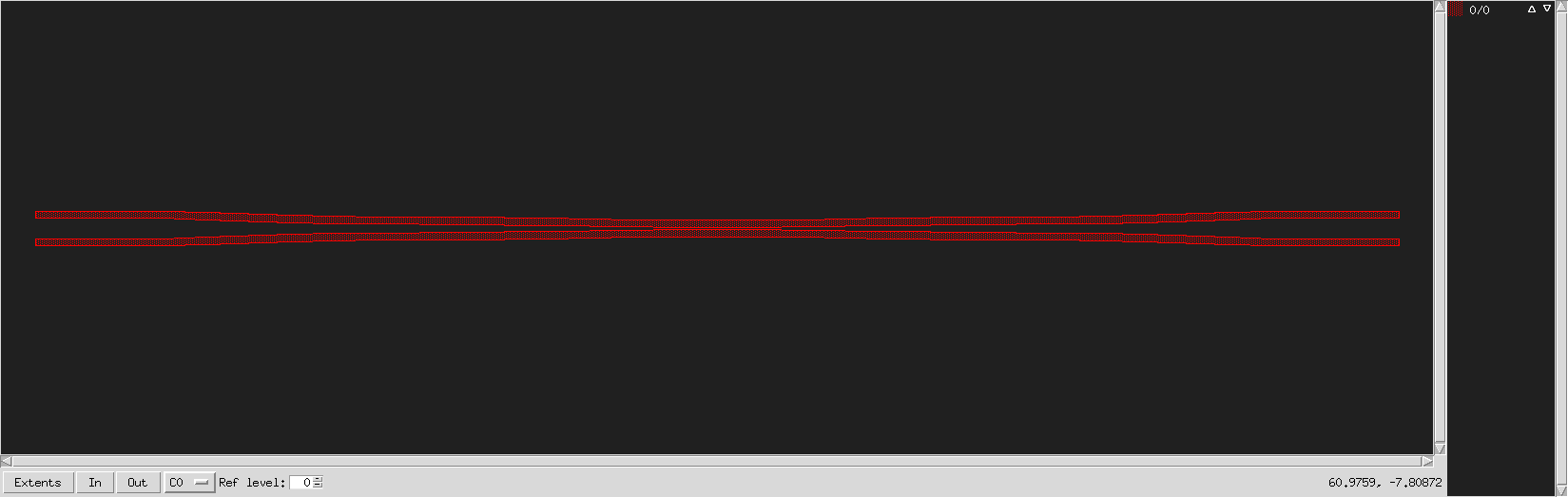
splitter
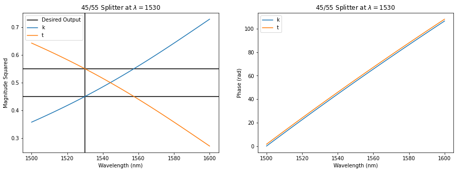
wavelength = np.linspace(1500, 1600, 100)
k = coupler.predict((1,4), wavelength)
t = coupler.predict((1,3), wavelength)

plt.figure(figsize=(15,5))
plt.subplot(121)
plt.axhline(.45, c='k', label="Desired Output")
plt.axhline(.55, c='k')
plt.axvline(1530, c='k')
plt.plot(wavelength, np.abs(k)**2, label='k')
plt.plot(wavelength, np.abs(t)**2, label='t')
pltAttr('Wavelength (nm)', 'Magnitude Squared', '45/55 Splitter at $\lambda=1530$', legend='best')
plt.subplot(122)
plt.plot(wavelength, np.unwrap(np.angle(k)), label='k')
plt.plot(wavelength, np.unwrap(np.angle(t)), label='t')
pltAttr('Wavelength (nm)', 'Phase (rad)', '45/55 Splitter at $\lambda=1530$', legend='best')
If you’d like this tutorial as a jupyter notebook, it can be found on github, here